Problem: Linear Relationship Between Variables

In an analytic geometry problem, we are studying the relationship between two variables x and y:

Definition of variables:

• x: Independent variable representing temperature in degrees Celsius (°C)
• y: Dependent variable representing temperature in degrees Fahrenheit (°F)

The following ordered pairs are known:

• Point 1: (0, 32) - When the temperature is 0°C, it equals 32°F (freezing point of water)
• Point 2: (100, 212) - When the temperature is 100°C, it equals 212°F (boiling point of water)

Based on this information, solve the following:

a. Find the equation of the line that relates y in terms of x

Determine the equation of the form y = mx + b that relates both variables.

b. Calculate y when x = 168

Substitute the value of x = 168 into the equation and calculate the corresponding value of y.

c. Solve for x in terms of y and calculate x when y = 78

Rewrite the equation to obtain x = f(y) and determine the value of x when y = 78.

d. For what value of x does x = y hold true?

Find the point where the line intersects with y = x.

e. Graph the relationship between both variables

Draw the graph of the function y = f(x), identifying significant points.

---

Tips

1. Identify key points: Use the given ordered pairs (x, y) to obtain the parameters of the line.

2. Determine the linear equation: Calculate the slope (m) and y-intercept (b) to find the equation of the line.

3. Evaluate the function: Use the equation to calculate specific values of the variables.

4. Solve the intersection: To find when x = y, set up a system of equations.

5. Plot the graph: Represent the relationship on a Cartesian plane, marking relevant points.

---

Solution

👉 View Solution

a. Equation of the line y = mx + b

We have two known points:

• (0, 32): x = 0°C, y = 32°F
• (100, 212): x = 100°C, y = 212°F

The equation of a line is y = mx + b, where:

The slope m is calculated as:

$$m = \frac{y_2 - y_1}{x_2 - x_1} = \frac{212 - 32}{100 - 0} = \frac{180}{100} = 1.8$$

The y-intercept b is obtained by substituting a known point into the equation:

$$y_1 = m \cdot x_1 + b$$ $$32 = 1.8 \cdot 0 + b$$ $$b = 32$$

Thus, the equation of the line is:

$$y = 1.8x + 32$$

Where:

• y represents the temperature in degrees Fahrenheit (°F)
• x represents the temperature in degrees Celsius (°C)

b. Calculate y when x = 168

Substitute x = 168°C into the equation:

$$\begin{align*} y &= 1.8(168) + 32 \\ &= 302.4 + 32 \\ &= 334.4 \end{align*}$$

The value of y when x = 168°C is y = 334.4°F.

c. Expression of x in terms of y

Starting from the equation y = 1.8x + 32, solve for x:

$$\begin{align*} y &= 1.8x + 32 \\ y - 32 &= 1.8x \\ x &= \frac{y - 32}{1.8} \end{align*}$$

This new equation allows us to calculate the temperature in Celsius (x) from the temperature in Fahrenheit (y).

Now calculate x when y = 78°F:

$$\begin{align*} x &= \frac{78 - 32}{1.8} \\ &= \frac{46}{1.8} \\ &= 25.56 \end{align*}$$

The value of x when y = 78°F is x = 25.56°C.

d. Value of x when x = y

To determine when x = y (i.e., when the Celsius temperature equals the Fahrenheit temperature numerically), set up the equality:

$$\begin{align*} y &= x \\ 1.8x + 32 &= x \\ 1.8x - x &= -32 \\ 0.8x &= -32 \\ x &= -40 \end{align*}$$

Thus, when x = -40°C, y = -40°F. The intersection point is (-40, -40).

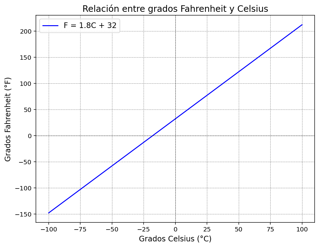
e. Graph of the relationship between variables

The graph is a straight line with slope 1.8 and y-intercept 32. Key points are:

• (0, 32): Intersection with the y-axis (when x = 0°C, y = 32°F)
• (100, 212): Second known point (when x = 100°C, y = 212°F)
• (-40, -40): Intersection with the line y = x (when the readings coincide)

---

Practical Applications

This problem illustrates how analytic geometry allows us to model linear relationships between physical variables:

1. Unit conversion: The equation enables transforming values between different measurement systems.

2. Linear modeling: It shows how physical phenomena can be represented using linear functions.

---